The usefulness of a Power duration curve.

Even a small hydro installation has a nightmarish cost. Making the decision to proceed with a project can mean having sleepless nights weighing up if the installation is likely to yield a reasonable return on investment. The key word here is  likely. Unfortunately being sure what an installation will yield is something of a black art which needs good data.

In this post, I want to give some data collected over the first two operating years of my project which help in thinking about how productive a hydro is.  It is data which, had it been available before committing, - an impossibility of course!, - would have been very useful in deciding whether to proceed or not.  Yet even without being able to have this 'hindsight beforehand', I hope that for someone who is still considering their scheme, looking at things in this way might stimulate thought about how viable their planned installation might actually be.

The data is presented in the form of a graph which combines in one curve the flow characteristics of my source and the practical challenge of making the most of that flow through timely nozzle changes. It has to be remembered that with a Powerspout you have to work at matching nozzles to the changing flow, and how good you are at doing that is reflected in the productivity of the installation.

The type of graph is technically called a cumulative frequency curve. It shows the percent of time that specified levels of power output were equaled or exceeded during two successive "Water years", each running from 1st October to 30th September.  Such curves are called Power-duration or Power-exceedance curves. Here it is:

What is immediately evident is that the two years are not the same: year 1 (blue) was wetter, peak power was limited in that year to 711 W, and generation was curtailed by me not being able to generate below 200 W.  Year 2, (red) by contrast, saw maximum generation increased to 750 W and generation was possible all the way down to 95 W*, thus extending the percent of the year when there was an output from 72% to 90%.

Despite these improvements, the total output for year 2, which is given by the area under the red curve, was very slightly less than for year 1.  The actual figures were 3,216 vs 3,350 kWh.

The point to note from this is that no single year is necessarily indicative of productivity.  Only several years without any changes to performance will give a true picture.

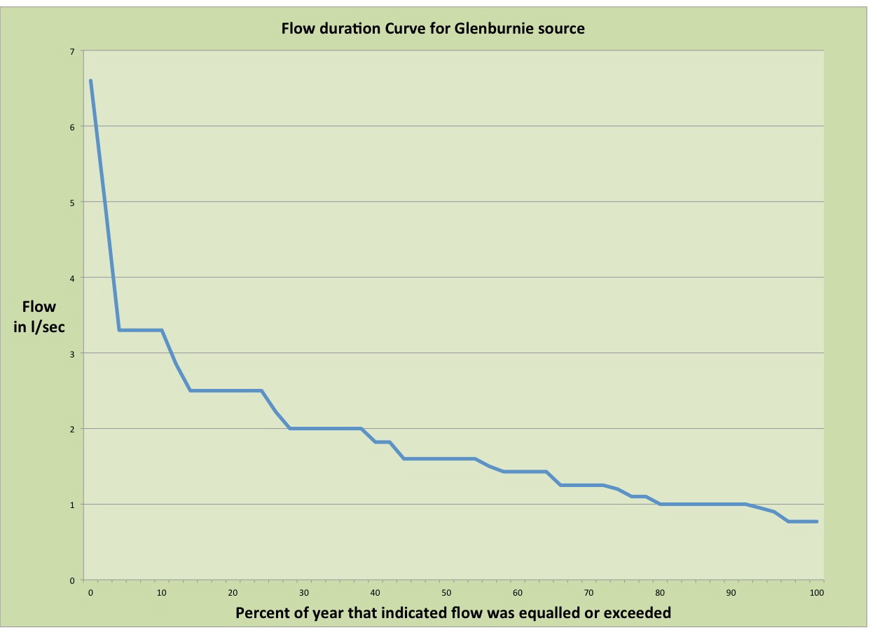
In general form, the power-duration curve is not dissimilar to another cumulative frequency curve namely the flow duration curve (FDC) for my source.  Clearly the two curves must be related to each other since the yearly pattern of power production must follow the yearly pattern of flow. Here is the FDC for my source, with data collected over 12 months back in 2009/10:

What is not intuitively obvious is that the 'bridging factor' which links the two graphs is the selection of what the 'design flow'** for the turbine should be at this site.

Choosing the design flow is a critical decision and needs to be considered carefully.  A matter which will influence the decision is how capable the turbine is at operating over flows less than the design flow.  As a general rule, opting for a design flow which your FDC indicates will be present for at least 50% of the year is a good starting point but immediately this should make you want to make sure that the measurements for your FDC were taken in a typical year.  There is no way of knowing that to be the case without extending the measurement period over more than a single year and amalgamating the results.  And that all takes a lot of time and effort!

In my case, I went for a design flow of 3 l/sec***. This was a bit ambitious: as the FDC shows, such a flow is only available for a little over 10% of a year and looking at the power duration curves confirms this: full power was only available for 10 % of year 2 and 20% of year 1, (but the latter was a very wet year).

Having opted for a rather high design flow, I then paid the penalty of not being able to keep operating at the lowest end of the flow range, - although by year 2 I had got this sorted by obtaining a reduced core stator for the drier months. And this highlights one of the advantages of the Powerspout system that not getting the design flow right first time can be corrected later by changing the Smart Drive stator.

So, to return to where we started, it is not easy to predict with reliability what the yield, and therefore the return on investment for your scheme will be, but it is possible if you have good flow data, especially if the measurements are gathered over several years.  

Never has it been more truly said "without data, all you have are opinions".  For those bitten by the micro hydro bug this might be re-written "without data, all you have are dreams" !

*    see link for explanation
**  design flow is the flow required for maximum rated output.  For owners claiming UK Feed in Tariff, it therefore determines what you give as your Declared Net Capacity (DNC)
*** this flow at 53 m net head produces 750 W out of the inverter into the grid

End of a "water year"

The end of September marks the end of what I call my "water year", by which I mean the twelve months which is centred on those months of the year when generation is maximal. 

Taking this span of time makes a graph of energy output look more tidy because each year begins and ends with the time of lowest output. Here is what this year's and last year's outputs look like superimposed on each other, blue for this year, red for last:

The totals generated in each of the two years were 3,350 kWh last year and 3,216 kWh this; not very different from each other. The pattern of peaks and troughs in generation are also not very different in the two years.

By the start of October I expect there to be too little flow to be generating so, because the turbine is shut down anyway, I generally set aside this time to do the yearly de-silting of the header tank.  This year however, as the blue line above indicates, a meagre daily output is still being produced, so today I have had to interrupt generation to get the job done:

The volume of water which has passed through the tank in the previous 12 months will have been in excess of 50 thousand cubic metres. With such a large volume, it is scarcely surprising that sludge collects but the amount I have scooped out today, when dry, would probably not amount to more than a tiny fraction of a cubic metre. So in fact the silt burden in the water is actually pretty low and a lack of abrasive wear on the pelton cups and nozzles reflects this.

My other bit of diary news is that I have just started on an experiment which has been stimulated by my last blog post entitled "Capping voltage".  There, I alluded to the problems of circuit board failures caused by dampness.  It has occurred to me that ventilating the electrical compartment with large volumes of moist air when there is a bulkhead kept cold by the temperature of the water on the other side, is a surefire recipe for creating wetness rather than reducing it.

So the plan is to seal the electrical compartment completely, pack all the spare space with
bags of silica gel, and see whether the humidity can be got down to a level where the dew point will never be reached however cold the surface of the bulkhead.  That's the plan but first there's a need to measure what the humidity and temperature are before the silica gel goes in. There's also the need to keep track of what the ambient temperature rises to in the compartment, especially as the level of power output increases over the coming months.  So I've made a little port hole through which to view a digital hygrometer / thermometer (£2.29 from ebay):

I'll report more fully later whether this 'sealed' approach reduces the wetness in the electrical side.